In Part – 1 we talked about linear algebra. This post will cover basic concepts of probability and probability distributions. Probably the most important mathematical topic needed in finance. Good news, its also not that hard. Everyone has a basic understanding of probability so none of this should be too hard. So let’s get started.
We will quickly go through a few basic concepts in probabilty, expected value, probability distributions.

1. Probability Basics: Probability is the likelihood of an event happening and is expressed as a value between 0 and 1. A probability of 0 means the event is impossible, while a probability of 1 indicates certainty. For any event A, its probability P(A) is given by:

P(A) = (Number of favorable outcomes) / (Total number of possible outcomes)

2. Conditional Probability: Conditional probability deals with the likelihood of an event occurring given that another event has already happened. For two events A and B, the conditional probability of A given B is denoted as P(A|B) and is calculated as:

P(A|B) = P(A ∩ B) / P(B)

3. Bayes’ Theorem: Bayes’ Theorem is a powerful tool to update probabilities when new information becomes available. It is formulated as:

P(A|B) = (P(B|A) * P(A)) / P(B)

where:

• P(A|B) is the posterior probability of A given B,
• P(B|A) is the likelihood of B given A,
• P(A) is the prior probability of A,
• P(B) is the prior probability of B.

4. Expected Value and Variance: Expected value (EV) is a crucial concept that represents the long-term average outcome of a random variable. For a discrete random variable X with probability mass function f(x), the expected value E(X) is given by:

E(X) = Σ (x * f(x))

For a continuous random variable with probability density function f(x), the expected value E(X) is given by:

E(X) = ∫ (x * f(x)) dx

Variance measures the spread or dispersion of possible outcomes around the expected value. For a random variable X, the variance Var(X) is calculated as:

Var(X) = E((X - E(X))^2)

Casino Problem

Let’s consider a simple casino game where you roll a fair six-sided die. If you roll a 6, you win $20; otherwise, you lose $5. The probability of winning is P(win) = P(rolling a 6) = 1/6, and the probability of losing is P(lose) = 1 – P(win) = 5/6.

The expected value of the game is:

(P(win) * $20) + (P(lose) * (-$5)) = (1/6 * $20) + (5/6 * (-$5)) ≈ -$0.83

A negative expected value implies that, on average, you would lose about 83 cents per game in the long run. This is typical of most casino games, where the house has an edge over players.

5. Probability Distributions: Probability distributions describe the likelihood of different outcomes occurring for a given random variable. Two essential distributions in finance are:

• Normal Distribution: The normal distribution is characterized by a bell-shaped curve and is commonly used to model financial phenomena like stock returns. It is entirely defined by its mean (μ) and standard deviation (σ).
• Lognormal Distribution: Asset prices often follow a lognormal distribution. If a random variable X is lognormally distributed with mean μ and standard deviation σ, then its probability density function is given by:

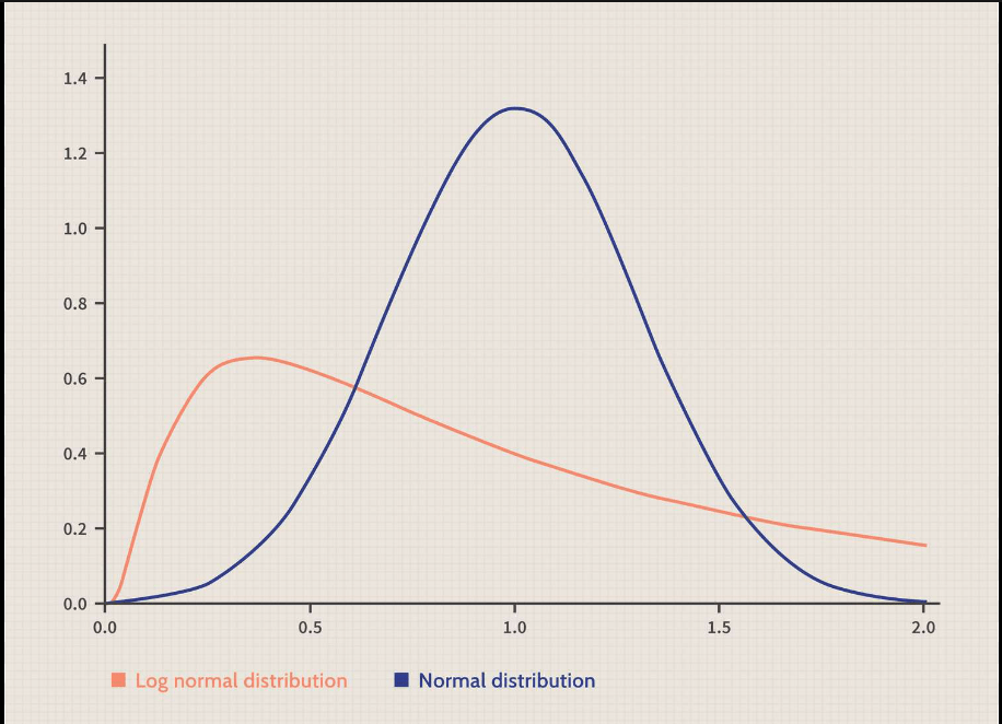
f(x) = (1 / (x * σ * √(2π))) * exp(-(ln(x) - μ)^2 / (2 * σ^2))

Ok thats enough with the boring parts. Now lets get to the fun stuff ….